Database Input/Output in Python

Data scientists commonly interact with relational databases. Answering a typical business question (e.g., what are our projected sales?) could involve learning which databases and tables hold the relevant data, constructing the query to pull the result set, and then post-processing the data in SQL, a spreadsheet, or Python. Where significant post-processing or analysis is required, getting the data into Python can be a winning option given the breadth of available standard and third-party libraries. Sometimes, it is further necessary to upload the processed data or derived artifacts from Python back into the database for consumption by others.

Databases typically support Python through modules following the Python DB API interface (PEP 249). This API, in my opinion, is more suited for software engineers than pandas-centric data scientists or data analysts. More appropriately, pandas allows for reading to and writing from dataframes via SQLAlchemy. I have observed in professional settings that mixing and matching Python DB API code with pandas + SQLAlchemy creates a mess. 

With a little creativity and foresight, it is possible to create a toolchain that is simultaneously simple, easy to use, and able to abstract away the details of using databases. In this article, I present my favorite way to interface with databases. An elegant twist on the pandas-SQLAlchemy API, it provides a drop-dead simple API and can slickly manage default connection settings. It can be readily extended to any database supported by SQLAlchemy. I build my case from examinations of the Python DB and the pandas-SQLAlchemy APIs. For an immediate look at my solution, please skip to Figure 11. 

The Python DB API

Python PEP 249 outlines a low-level API to communicate with a generic database management system as described by computer science. It standardizes database connections, database transaction management (e.g., commits and rollbacks), and the operation of cursor objects. A database cursor is like an iterator object that handles row traversal as well as retrieval, insertion, and deletion.

Typical usage of the Python DB API involves the following steps:

• Load the package for a particular database (SQLite, MySQL, etc.).
• Establish a connection by specifying the relevant server, database name, database schema, and any required authentication credentials.
• Extract a cursor object from the connection.
• Run the query or SQL command with the cursor's execute method.
• If retrieving data, call one the of the cursor's fetch methods (e.g., fetch_all).
• Convert the result set into a Python dataframe.

Figure 1 exemplifies this workflow for a MySQL database.

Figure 1: Reading data from MySQL using the Python DB API.

Writing back to the database also involves the cursor object. If the table does not exist, it needs to be explicitly created from the cursor. One must then write and apply the insert statements through the cursor. Figure 2 shows an example for MySQL.

Figure 2: Creating and writing a database table with a cursor object.

The pandas-SQLAlchemy API

The Python DB API will likely feel unintuitive to data scientists and analysts lacking a significant computer science background. Data analysis in Python commonly incorporates pandas dataframes, and, luckily, the pandas project provides support for relational databases via SQLAlchemy. The pandas.read_sql function reads a query result set into a dataframe. The DataFrame.to_sql method pushes the contents of a dataframe to a database table. No cursor management or detailed understanding of database operation is required.

The most involved aspect of using a database with pandas is initially hooking the database up to SQLAlchemy. This configuration begins with the SQLAlchemy engine, which is aware of the type of database being used, where the database is located (e.g., web versus memory), and any authentication credentials. It also allocates resources (a connection pool) to manage database connections. Figure 3 defines an example engine for a MySQL database running on localhost. Note the database username and password are retrieved from the environment.

Figure 3: Connecting to a MySQL database via SQLAlchemy.

With the connection in hand, the pandas utilities are easy to use. Figure 4 repeats the same retrieval from Figure 1, with much less code. 

Figure 4: Using pandas.read_sql to query the database.

Uploading to the database is likewise easier. Figure 5 re-implements the upload in Figure 2. Note that the data is formatted as a dataframe instead of insert statements.

Figure 5: Writing a new database table with Dataframe.to_sql.

Additionally, the SQLAlchemy engine allows for execution of SQL commands. A little more work, it involves getting a connection from the engine and converting the SQL statement into a SQLAlchemy text object. Figure 6 shows an example helper function and its usage. Note that the commit method is called after the command is executed. Following the Python DB API, the connection object does not assume the changes will be automatically committed (any auto-commit feature supported by the underlying database must be turned off by default).

Figure 6: Executing SQL commands with SQLAlchemy.

To simplify the pandas-SQLAlchemy API, one could write helper functions that abstract away the details of SQL read, write, execute operations. Figure 7 provides such an example. Note that the pandas functions support several important kwargs; any optional arguments are passed through to pandas.

Figure 7: Helper functions for the pandas-SQLAlchemy API.

These helpers are a reasonable way to engage with a database in Python. They are agnostic to the type of database since anything supported by SQLAlchemy is also supported. Less than ideal, however, is that the SQLAlchemy engine must be explicitly created and passed into the functions every time. 

My dbio (database input/output) module

The next logical step is to represent a database connection as a custom class having 1) read, write, and execute methods and 2) a SQLAlchemy engine stored as an attribute. This design allows object methods to already have access to the engine, saving the user from repetitively passing in the engine with each call. For extra convenience, the SQLAlchemy engine is automatically created on initialization without the user having to remember the specific details for connecting to a particular database (e.g., Figure 3). I put this idea into practice through my own Python package called dbio (database input/output).

There were two important design choices I made. First, I built a base class called _Connector that defines the read, write, and execute methods. These methods are similar to the helper functions in Figure 7 but omit the function argument for the engine; they instead reference the engine attribute of the class. The other difference is that the read method optionally performs a memory optimization procedure called downcast that shrinks data to the smallest possible datatype while preserving all the information. For example, a 64-bit integer (int64) might convert to int16 without any downside. In my experience, the biggest memory savings comes from converting strings to the pandas categorical type.

The constructor of the base class needs to be aware of the database server, default database name, and default schema; these are set as object attributes. Figure 8 shows how the base class initializes.

Figure 8: The base class in dbio. Not pictured: the read, write, and execute methods.

The second important design decision was that supported databases each have their own derived class that inherits read, write, and execute from the base class. The constructor for the derived class is aware of all the parameters needed to get the database connection and sets sensible defaults; on initialization, the server, default database, and default schema are passed to the base class constructor (super().__init__). Each derived class also contains a get_engine method that sets up the SQLAlchemy connection given the input parameters; note that get_engine is called automatically by the constructor. 

Figure 9 shows the subclass for a SQLite connector. Note that with SQLite there is no database server or schema (the database is a file).

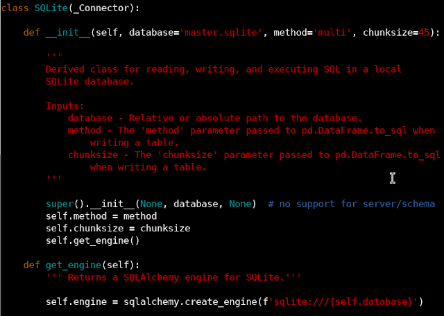
Figure 9: The SQLite derived class.

The derived class for MySQL (Figure 10) is slightly more complicated. In addition to the database server, the username and password credentials must also be handled. Accordingly, the get_engine method takes more arguments. Note that MySQL also does not support a schema.

Figure 10: The MySQL derived class.

Finally, Figure 11 shows how the MySQL database operations look when they are done through a dbio connection object (cobj). This version is significantly shorter because of all the boiler plate code abstracted away by dbio. With this tool, a data scientist can focus more acutely on the project without sacrificing any ability to interact with a database.

Figure 11: Sample usage of dbio. The connection object (cobj) provides the read, write, and execute methods.

Building a Python package

For ease of re-use and portability, I have created a dbio Python package and installed it on my own system in a virtual environment. The current standard for creating a package is to use a pyproject.toml file. This configuration file defines the name of the package, version, dependencies, and other details such as how the package will be built. Figure 12 shows the settings for dbio. Note that I'm using setuptools. Also, the package version is set dynamically from an __init__.py file. 

Figure 12: The pyproject.toml file for the dbio project.

Final remarks

Dealing with databases in Python is a lot more fun with dbio! To date, I have written three versions of dbio. The one described here is my own personal version (and is available upon request). Other versions I have written professionally support SQL Server, Snowflake, and Denodo. Using dbio with an unsupported database does not require modifying the package. One could import the _Connector base class and write their own local module for any other database.

Certain customizations to dbio may make sense depending on the details of the development/production environment. Regarding database parameters, for example, the default database and schema could be set to whatever is appropriate for the broader team. If warranted, a derived database class need not even depend on SQLAlchemy. Snowflake provides its own support for pandas dataframes that may in some cases be superior to going through SQLAlchemy. In this case, the read, write, and execute methods can be defined in terms of the vendor-provided tools without changing the dbio API.

In contrast to the MySQL connector presented here, where the user is responsible for providing the credentials, authentication may be carefully automated. For example, when a team is operating with a common 'service account', the account name could be set as a default parameter in the database connector, and the corresponding password (or whatever) could be securely retrieved from, e.g., a vault. Some vendors, such as Snowflake, support single sign-on through a web browser. In this case, the username could be automatically retrieved through the environment, and the browser authentication could be triggered automatically as part of the get_engine method. 

Using Database Search and Email In LangChain Agents

In the previous post about prompt engineering for large language models (LLMs), I demonstrated that ChatGPT could navigate word math problems if prompted suitably. In this post, I explore ChatGPT's ability to reason about tabular data, including relational database tables. The source code use in this article is available here. 

Pizza time! (No turtles please)

The DeepLearning.AI short course on prompt engineering culminates with the demo of a pizza OrderBot. The bot is able to answer questions about the menu, gather the order, and summarize the whole thing at the end, complete with the correct total price. The menu in this example is represented in plain text within a system role message (Figure 1). 

Figure 1: System role message with menu

Figure 2 shows an example of a complete order executed by the bot. 

Figure 2: Sample order

One well-known problem with LLMs, however, is their tendency to hallucinate. Asking about details not provided in the prompt causes the model to make up details based on its original training. This can be dangerous in production applications because even inaccurate responses can sound reasonable. Figure 3 shows examples of hallucinations about details not provided in the pizza menu. 

Figure 3: Hallucinations

The errors in these specific examples are fixable by adding more details (diameters of pizzas, sizes of drinks) to the menu text in the prompt. Fool-proofing the menu would be an iterative process that could potentially cause regressions as menu complexity increases.

Querying structured data

Here, I explore if hallucinations are reduced when the menu is structured in SQL tables instead of plain text. I hypothesize that well-chosen table and column names would act as metadata to help the LLM understand how and whether to answer a given question. 

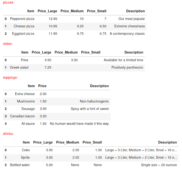
To set up the database, dataframes were made for each category of item (pizza, topping, side item, and drink). They were first prototyped as pandas dataframes and then loaded into a SQLite database with SQLAlchemy. The table schemas consist of the item name, price, and item description. Figure 4 shows the full content of the tables. 

Figure 4: Pizza menu database

ChatGPT was connected to the database via LangChain, an exciting new open-source framework for incorporating LLMs into applications. The project provides modular components for a) connecting LLMs to external data sources and b) accomplishing higher-level tasks like Q&A sessions. The components can be chained together to create arbitrarily complex applications. The short, and currently free, LangChain course from DeepLearning.AI provides an accessible and comprehensive introduction.  

LangChain provides a SQLDatabaseChain component for querying data in any database compatible with SQLAlchemy. The tool implements established best practices for prompting an LLM to write SQL queries, although further customization of the prompt is possible. The minimal steps for setting up the SQLDatabaseChain include connecting to the database and initializing an LLM (Figure 5). After experimenting with my own prompt, I adopted the default prompt. 

Figure 5: Using SQLDatabaseChain

I expect the SQL chain to perform at least as well as the version with the plain-text menu, so I start by presenting the three inputs that caused hallucinations in Figure 3. Impressively, the SQL chain answers all the questions correctly and without hallucinating false details. Figure 6 shows the results. Some of the output remarks (e.g., "The sizes and their corresponding dimensions are not provided in the database.") are not necessarily things that should be shown to end users, and prompting the model to use a different tone would be worthwhile.

Figure 6:  Questions now answered correctly with a SQL database

Some comments are in order:

• These examples demonstrate the ability of the LLM to examine the data schema and write the SQL needed to efficiently solve the problem. In each case, the SQL chain is following the process specified in the prompt: identify the question, write the SQL query, get the query output, and formulate the final answer. 
• In the first example (number and sizes of pizza), the LLM inferred from the Price_Large, Price_Medium, and Price_Small fields that there the three pizza sizes are Large, Medium, and Small. It did not confuse the prices as measurements of size (although, see below where this does happen), and it correctly stated that information on dimensions is not available.
• In the second example (number and sizes of bottled water), the LLM found only one row and read from the description that the size is 20 ounces. The Price_Medium and Price_Small columns were NULL, but it is not clear this was used in the answer. Asking a related question on the number, size, and cost of Coke returns a detailed and correct answer, which is reassuring. 
• In the third case (Greek salad as a topping), the LLM joined the pizzas and toppings tables together, found no rows where 'Greek salad' was a topping, and concluded it was not possible.

As impressive as the above results are, the LLM still gets fooled by seemingly simple questions. When asked simply about the diameters of pizza size (which was answered correctly above as part of a longer question), the LLM confuses the price values for pizza dimensions. When asked a second time and reminded that the price values are dollars and not dimensions, it correctly reports that it cannot answer the question.

Figure 7: Confusing dollars with inches

As a final example, I ask about the size of a small cheese pizza topped with mushrooms and sausage. The chain manages to join the pizzas and toppings tables together in a way that returns 0 rows (Figure 8). This is disappointing since the original chatbot with the text menu could answer such a question. Non-invasive ways to fix this text-to-SQL brittleness include customizing the prompt instructions and/or including sample rows in the prompt. 

Figure 8: Incorrect price quote

In this case, I tried out the SQLDatabaseSequentialChain which first examines the schema to decide which tables are relevant and then calls the SQLDatabaseChain for the relevant tables. The result is correct and is shown in Figure 9. The better outcome is not a fluke. The sequential chain consistently outperforms the simpler chain in repeat trials. It might be that the sequential chain is giving the LLM a more detailed examination of the table schemas, so that it is able to write more relevant SQL.

Figure 9: Correct price quote

Better ingredients, better PizzaBot

Using the lessons learned above, I now assemble a new pizza OrderBot more robust than the one above (Figures 1-3). In addition to working off a database representation of the pizza menu (Figure 4), I would like the bot to be able to send a summary of the order to the user's email. The bot will have to converse with the user in real-time and know when to access tools for searching the database and sending the email. 

The LangChain Agent interface is able to select which, if any, of the available tools should be called based on the user input. Referencing detailed examples (especially this one) from LangChain's documentation, I was able prototype the desired functionality in my own custom agent.

The final solution consists of the following components: 

• A conversational agent (langchain.agents.ConversationalAgent) with a custom prompt spelling out its role as an OrderBot. 
• Conversation memory buffers (langchain.memory.ConversationBufferMemory, langchain.memory.ReadOnlySharedMemory)
• A SQLDatabaseChain for querying the pizza database (see Figures 5 and 9 for details)
• Two instances of LLMChain: one for the agent and one for producing the order summary. 
• A Custom email function: input is a single pipe-delimited string containing order summary and recipient email address.
• An underlying LLM (gpt-3.5-turbo)

The agent needs access to tools for database search (SQLDatabaseSequentialChain), order summary (LLMChain), and sending emails (custom function). The order summary tool is just an LLMChain with a custom prompt. Given the chat history (via an instance of ReadOnlySharedMemory), it will summarize the name and price of each item, as well as the total price. The code for customizing this chain is shown in Figure 10.

Figure 10: LLMChain order summary tool

The tools are set up as a list of langchain.agent.Tool objects. Each Tool instance knows its own name (e.g., 'Menu Search'), what function it points to, and has a text description the LLM parses when deciding which tool to call. Figure 11 shows the final configuration of the tools. Note the Order Summary tool additionally has the return_direct=True parameter, which returns the output of the tool directly to the agent (otherwise the LLM would read and rephrase the order summary).

Figure 11: The OrderBot's tools

The Send Email tool (Figure 12) is the most complex. I specify in the description that the input is one pipe-delimited string containing the order summary text and the user's email. The send_message function then parses the substrings before it formats the email. Correct output from Send Email requires that Order Summary be successfully called first.

Figure 12: How emails are sent

To make the OrderBot more self-aware about its role in the pizza ordering process, the ConversationalAgent's prompt needs to be edited. The default prompt includes a prefix, a description of available tools, and a suffix. I edit the prefix to explain the OrderBot's function. The tool list is automatically populated from the existing list of tools. The suffix has placeholders for the chat history, user input, and a scratchpad for the agent to compose a response. Figure 13 shows the code for updating the prompt while Figure 14 shows the fully formatted prompt template.

Figure 13: Customizing the agent's prompt

Figure 14: Final agent prompt template

As shown in Figure 15, the final agent chain (agent_chain) comes from bringing the components together in the langchain.agents.AgentExecutor.from_agent_and_tools method. Note, custom agent (agent) gets the custom prompt (agent_prompt) by way of an LLMChain. To prevent any parsing errors from causing a problem, the agent_chain.handle_parsing_errors parameter is set to True.

Figure 15: Defining the final agent (agent_chain)

The pizza OrderBot is finally ready to use (e.g., agent_chain.run('What pizzas are available?')). The OrderBot turned out to be friendly, helpful, and addressed me by name. It could answer questions about the menu from the database exactly as shown above. Figure 16 shows an example of a correctly handled order. Figure 17 shows the email summary that was sent. 

Figure 16: Sample conversation

Figure 17:  Email order summary

I am largely satisfied with the prototype OrderBot. I experienced some difficulty formatting the email content. Attempts to format the order summary as an HTML table did succeed consistently. Getting the LLM to use some HTML (e.g., line breaks) would be helpful for summarizing long orders.

Summary

In this article, I have examined ChatGPT's ability to query and reason about tabular data. I found some indication that tabular data (a pizza menu) stored as plain text can inspire LLM hallucinations. Splitting the menu into multiple database tables seems to mitigate, but not eliminate, hallucinations. Finally, a prototype OrderBot capable of reading from a database and sending an email was presented. The OrderBot code is a template that can be repurposed for other custom chatbots.

Note: This article was produced with LangChain 0.0.220 and ChatGPT gpt-3.5-turbo-0301.

An Introduction to Prompt Engineering for ChatGPT

It has been over 6 months since the public release of ChatGPT in November 2022. The service was an immediate hit. As the most sophisticated example of a large language model (LLM) to date, the Internet wasted no time in interrogating its capabilities. As LLMs mature, dependence on such AI in daily life could increase dramatically.

The interactive web app is the easiest way for users to leverage ChatGPT right now. Novel future applications will require integration into devices or services having access to cloud-hosted models through APIs.

OpenAI provides a ChatGPT API for Python and node.js, and the broader community maintains libraries for other languages. Apart from the official documentation, another great way to learn is through the short ChatGPT courses currently on offer for free by DeepLearning.AI. As a new user to the API, the most surprising takeaway from the courses was that basic Python skills combined with the OpenAI API are sufficient to build new, ChatGPT-powered systems.

This article memorializes the key lessons I learned about using OpenAI's ChatGPT API. It is intended to be a reference for myself and a tutorial for new users to the API. The resources from the short courses are available here, and the original examples produced for this article are here.

Basic setup and authentication

Getting started in Python requires two steps:

1. Installing the OpenAI module (pip install openai);
2. Acquiring an API key.

In code, the API needs to be aware of the API key. It is not recommended to hard code the key in the code itself, and such code should never be submitted to a public repository. A simple alternative is to store the API in a local file called .env and to use the dotenv module (pip install dotenv) to detect the file and load the key as an environment variable.  Figure 1 provides an example of how this can work:

Figure 1

Your first API call

Everything is now in place to start talking to ChatGPT. The ChatCompletion object creates a model response given a chat conversation. The chat conversation can be a single prompt or an entire chat history. In either case, the model parses the text and returns the most likely response. 

Figure 2 shows a helper function for obtaining the response for a single prompt (i.e., input message). Follow-up calls with different messages will be treated as different conversations. This is unlike the web app where history is preserved within each separate conversation.

Figure 2

The model argument configures which language model to use. The GPT-3.5 model family can generate natural language and computer code. Of these, gpt-3.5-turbo is recommended as the best performance per cost ($0.002 per 1K tokens, or approximately 750 words). The full list of available models is here. 

Secondly, the temperature argument controls the randomness of the response.  Allowable values are in the range [0, 2] and lower values correspond to less randomness.  Even at temperature 0, however, the model is mostly but not entirely deterministic.

The ChatCompletion call returns a particular kind of object (openai.openai_object.OpenAIObject) that contains the desired response plus additional meta data.  From the full output (response), we want only a small piece, response.choices[0].message["content"]. Figure 3 shows the full response and, at the very bottom, the desired relevant output.

Figure 3

The input prompt can be 'engineered' to maximize the utility of the single output message ("prompt engineering" is an emerging new skill in the application of LLMs). For example, we can tell ChatGPT to include more fields (year written, short summary) and to format the output as a JSON object. If we were interested in using this as a Python object, we could convert with Python's JSON utilities.  See Figure 4 for the result.

Figure 4

This example highlights the importance of writing clear and specific instructions, which can include asking for structured output.

Multi-message chats

The ChatGPT model is stateless. Producing coherent conversations requires that at least some previous messages in the conversation be uploaded every time (increasing the number of tokens used) for the model for generate the next most likely response. The illusion of continuity is created at the expense of each API call becoming slightly more costly as a conversation unfolds.

In the above get_completion function (Figure 1), the user prompt is formatted into a list (messages) of dictionaries. Each dictionary encodes one message (content) and the source (role), which indicates the source of each piece of dialog. Role has one of three values: user (the human), assistant (the chatbot), and system (context for the assistant not meant to be visible to the user).

Figure 5 demonstrates passing multiple messages to the ChatGPT. In this case, the system role is instructing the assistant that is is to speak like Shakespeare, and that the user cannot override that style.  The user then asks to hear a joke in a different style. The model apologizes that it must stick to the specified original style and then delivers a four-line joke complete with rhyme.

Figure 5

With this in mind, it is surprisingly simple to create a chatbot within a Jupyter notebook. In the example below (Figure 6), I have attempted to recreate the famous Duck season versus Rabbit season debate between Bugs Bunny and Daffy Duck. The Assistant is Daffy Duck, and the User is Bugs Bunny. Elmer Fudd is standing by with his rifle. The chat window widget is a panel widget. Source code for the chat is here.

Figure 6

Reasoning about math word problems

In this next section, let's explore whether ChatGPT can handle word problems. The answer is "yes, if prompted suitably".

I developed exercises that present options for eating out versus cooking at home. The model is supposed to evaluate each option and decide which is cheaper. In addition to choosing the right option, the model also verbalizes the cheaper option and outputs the amount saved daily and annually.

Figure 7 shows my first attempt (V1) at a prompt for the base case (eating out costs 15 dollars per meal while eating at home is 5 dollars per meal; the user always eats three times a day). ChatGPT gets the right answer (eating at home; annual savings of 365*3*($15 - $5) = $10,950). Note that it is useful in many contexts to inform the model that the user's prompt will be specially marked by delimiters such as triple backticks (```).

Figure 7

Asking the same question in a second way reveals a weakness in the prompt.  In Figure 8, I present the cost of eating at home in units of cents (1/100 dollars), hoping to confuse the system.  The model ends of doing the calculation in units of cents, and the output savings are quoted in cents. While this is not technically wrong, it can be considered incorrect since it is atypical to express amounts exceeding one dollar in cents.

Figure 8

Figure 9 shows the second version (V2) of the prompt in which the model is told to calculate in dollars and make the decision based on the total number of dollars spent per day. The description for the output also reminds the model that daily and annual savings need to be presented in dollars. This version of the prompt produced the expected output.

Figure 9

After just two iterations, the results were promising. However, prompts are ideally tested on a battery of examples. The two prompts were tested on the set of five examples described in Table 1. Examples 1-3 mix dollars and cents. Example 4 mixes total cost per day and the total cost per meal. Example 5 does the same while mixing dollars and cents too.

For the model to pass each example, it had to choose the right option (a or b) and calculate the total annual savings in dollars. An answer that chooses the right option while getting the units wrong is only half correct.

The total score for each prompt comes from adding the scores for the individual examples. The first prompt (V1) scored 40% while the second prompt (V2) scored 100%! Table 2 shows the detailed scoring for each test.

Let's examine in detail what V1 got wrong. 

1. Half of Example 1 is wrong because the output savings is not in dollars. 
2. In Example 2, the letters associated with each choice are flipped, and choice (b) is listed before choice (a). See Figure 10 for details. ChatGPT outputs the wrong letter (a) and calculates 0 zero savings. The prompt was apparently confused by the choices not following alphabetical order.
3. All of Example 3 is wrong because the model outputs a blob of Python code instead of numbers.
4. Example 4 is fully correct. 
5. Example 5 partial credit is awarded because the units are wrong.

Figure 10

How is V2 guiding to model to get the right answer every time? The prompt is is spurring ChatGPT to write it's own robust Python code that gets the right answer every time. At the end of the code blob (Figure 11), the model is producing is constructing a dictionary in the desired output format.

Figure 11

If this prompt were included in an a user-facing app, the tests should be repeated periodically to make sure that there is no regression in performance as the prompt or underlying LLM changes. If V2 begins to fail as further examples were added, the decision to e.g., standardize the currency amounts to dollars might have to be made.

Conclusion

This article has demonstrated important strategies in designing prompts for ChatGPT LLMs.

1. Helpful tactics for improving prompts include providing clear and specific instructions, using delimiters (e.g., ```) to mark user input, telling the model to work through explicitly defined steps, and asking for structured output.
2. Prompt development is iterative and is best done in a systematic, test-driven way. Test criteria can be explicitly as shown here. It is also possible to have the LLM grade it's own response (not discussed here).
3. For prompts under active development, tests should be re-run periodically to prevent regressions in system performance.
4. Tuning applications of LLMs is very different from the process needed for other AI models.

Hopefully this article helps and inspires you to start building new applications with ChatGPT!

Graph Analysis of the Leaked Democratic National Committee Emails

Graphs are constructs used to model the pairwise relationships between objects. Graph theory, the organized study of graphs, is a rich topic with applications to many problems in the physical, biological, social, and information sciences. In this first post on graph theory, I use a graph to visualize the sender-recipient relationships within the emails stolen from the Democratic National Committee (DNC) and published in searchable form on WikiLeaks. The details of how I retrieved the emails, parsed them, and created the graph are summarized. I also quantitatively characterize the graph and discuss community detection within the network. Finally, I end with a demonstration of the R Shiny application I have deployed for playing with this dataset. The Shiny application source code plus the final graph are available on Github.

Email Extraction, Transformation, and Loading into Graph Format

The emails are stored in EML format at addresses of the form $\texttt{https://wikileaks.org/dnc-emails/get/i}$ where $\texttt{i}$ is an integer between 1 and 22,456. The emails were downloaded one-by-one from WikiLeaks using the powerful tool $\texttt{curl}$. The downloader script I prepared is available on Github. It took about 6 hours to retrieve all 22,456 emails (1.7 GB).

The emails were parsed using the $\texttt{email.parser}$ package built into Python. Given a file object for an email, the $\texttt{HeaderParser}$ class returns the header data in key-value pairs. I extracted the sender, recipient(s), and subject line from the header of each email and then did some text preprocessing (e.g., converting letters to lower case, stripping white space) before writing this information into ASCII files (dnc_subject-out.tab, dnc_from-out.tab, dnc_to-out.tab) available on Github.

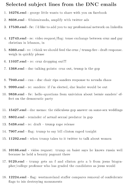
While the subject lines will not be used in the graph analysis, it is interesting to briefly consider them because they provide clues about the email contents. A wide variety of topics, including some surprising ones, are discussed. Figure 1 lists subject lines that caught my attention.

Figure 1: A sample of subject lines in the DNC emails.

The DNC emails are described on WikiLeaks as having come from seven email accounts. The numbers of unique email senders (1192) and recipients (1169) in this email dataset, however, are much larger than seven! The total number of unique identifiers among all senders and receivers is 1777. This includes two identifiers labeled as 'None' and 'undisclosed-recipients' representing one or more unknown email addresses. Some of the identifiers are phone numbers or generic labels like 'wireless caller'.

The details of email communication between all unique email addresses can be represented in an NxN matrix $M$ such that the value of $M_{ij}$ is the number of emails $i$ sent to $j$. If $j$ wrote back, then $M_{ji}>0$. Cells along the diagonal ($M_{ii}$) are positive and nonzero if people email themselves. $M$ intuitively translates into a directed graph. Every cell $M_{ij}$ represents a potential graph connection (or edge) from vertex $i$ to vertex $j$, which only exists if $M_{ij}>0$. If $M_{ji}>0$ also, then a parallel edge exists from vertex $j$ to vertex $i$.

For simplicity, I chose to represent the DNC email network as an undirected graph. This means an edge between vertices $i$ and $j$ exists if $M_{ij}>0$ or $M_{ji}>0$. I discarded the emails where no sender (N=144) or receiver (N=223) information was available (i.e., emails having 'None' or 'undisclosed-recipients' as the sender or recipient), which removed 26 vertices from the graph.

There are various graph analysis packages in Python (e.g., graph-tool, igraph, NetworkX). I chose igraph because it is simultaneously available in R as well as Python. The python-igraph interface is intuitive to use, and it is quite fast for my purposes.

Taking advantage of igraph support for vertex and edge attributes, I assigned each vertex a 'name' attribute to store an email address string. I also gave the edges an attribute ('dir') to represent one-way versus two-way communication and another attribute ('mag') to represent the number of emails exchanged. There are 1751 vertices and 3976 edges in the final graph, which is available on Github in GraphML format. One can immediately explore the DNC email network by importing this graph into his or her favorite graph analysis tool. My Python scripts on Github (mkGraph.py, analysis.py) demonstrate how to interact with the graph.

Graph Visualization and Community Analysis

The first step in appreciating the complexity of the DNC email network graph is visualization. Fortunately, igraph provides a powerful but straightforward plotting interface. With experimentation, I found force-directed algorithms produced the most aesthetically pleasing result. Figure 2 shows the graph as drawn with the Fruchterman Reingold force-directed layout. Each circle is a vertex representing a unique email address. Gray edges mean one-way email communication while orange edges indicate two-way communication. The center of the graph is crowded with many crossing edges. At intermediate radii are fan-like structures, or "communities", in which many nodes that share a common email connection are sparsely connected to outside nodes. At the outskirts are nodes that have only one email connection or that just email themselves, creating a loop.

Figure 2: The DNC email network plotted with a force-directed layout algorithm. Gray edges mean one-way email communication and orange edges mean two-way communication. Vertices that are slightly enlarged have degree $\geq 125$ and are discussed in the text below.

Next, let's consider the basic properties of the vertices and edges. Vertex degree refers to the number of edges adjacent to a vertex (note, a loop adds 2 to vertex degree). The histogram of vertex degree has a steep drop at low degree and a long tail at higher degree. The majority of vertices (1127/1751, 64.4%) have degree$=1$. Significantly less (17.1%) have degree$=2$. About 9.7% have degree$\geq7$, and the top 5.0% have degree$\geq18$. The top three vertex degrees are 476 (comers@dnc.org), 471 (mirandal@dnc.org), and 274 (kaplanj@dnc.org).

Figure 2 gives the impression that most email communication is unidirectional. Indeed, 64.4% (2641/3976) of edges in Figure 2 are gray. Figure 3 gives insight into the number of emails typically exchanged (either way combined) between individuals. The majority of email exchanges are relatively brief. About 35.9% of graph edges signify the exchange of a single message. Approximately 66.9% of graph edges represent an exchange of $\leq4$ messages. Roughly 9.9% of edges correspond to email exchanges $\geq23$ messages. The top three email exchanges involve comers@dnc.org mailing himself (512 messages), mirandal@dnc.org and paustenbachm@dnc.org mailing each other (665 messages), and dncpress@dnc.org mailing itself (1492 messages).

Figure 3: The cumulative fraction of graph edges as a function of emails sent per edge in the DNC email network graph. The bins are five emails per edge wide.

Figure 4 is a similar plot showing how the cumulative fraction of confined edges increases with the maximum allowed vertex degree. The curve in Figure 4 rises smoothly initially but then begins to show step features corresponding to the community structures in Figure 2. The community structures arise because vertices of intermediate and high degree connect to many vertices that are in turn sparsely connected. A significant fraction (34.1%) of the graph's edges are connected to one or more of the five vertices with degree $\geq 125$. The legend of Figure 4 lists the persons associated with these most influential vertices, and the same five vertices are also distinguished in Figure 2 as being slightly enlarged and having vertex colors matching the lines in Figure 4.

Figure 4: The cumulative fraction of edges originating and terminating within vertices as a function of vertex degree. The vertical lines mark the five highest-degree vertices to which 34.1% of the graph's edges connect.

While Figure 4 associates the most highly connected nodes with separate communities, a more sophisticated approach is required to find all communities and determine their member nodes. The study of community structure in graphs is an active field, and there are many algorithms implemented in igraph for this purpose. From the available algorithms in igraph, I have chosen the Louvain Modularity (LM) method. Modularity is a scalar measure of graph structure; positive modularity means vertices are more densely interconnected than expected by chance. LM partitions communities in a bottom-up, hierarchical way that maximizes the modularity of the graph. LM is suitable even for networks with over 100 million nodes, and it is fast and effective compared to competing algorithms.

The LM algorithm finds 47 communities in the DNC email network and reports a modularity of 0.6 (on a scale of [-1, 1]). Over half (36/47) of the communities have just one or two members, and these small communities are the isolated vertices in the graph outskirts. The other 11 communities have between 5 and 429 members. Figure 5 redraws the graph with color coding for the vertices in the 11 largest communities. As intuitively expected, the largest fan-like structures are separate communities. There are also multiple communities coexisting in the center of the graph where it was hard to see structure in Figure 2.

Figure 5: An alternate rendering of Figure 2 with color coding for the 11 largest communities as discovered by the Louvain Modularity algorithm. The black vertices at the outskirts represent small communities with only one or two members. The enlarged nodes have the highest vertex degree within their communities.

Table 1 lists the 11 largest communities in descending order of the number of community members. The second column names the person with the most email connections (i.e., highest vertex degree) in each community; these people may perhaps be considered as "community leaders", and they appear as enlarged nodes in Figure 5. The third column of Table 1 indicates the color of the community in Figure 5. The five vertices with degree $\geq125$ highlighted in Figure 4 turn out to be community leaders in Table 1. The number of nodes per community roughly, but not perfectly, increases with the vertex degree of the community leader.

This graph analysis has demonstrated how to find substructure in a graph and further how to identify the most prolific individuals within network communities.

Interactive Shiny Web Application

Shiny is a web application framework for the R programming language. It is powerful while still being simple to use, and its attractive widgets make for very nice looking applications. I have designed a Shiny application that provides interactive visualization of the DNC email network. This application incorporates the R version of igraph and uses the qgraph package for plotting. My approach was to prototype all the intended functionality with python-igraph first, because it is more intuitive to use, and then port it over to the R version. It is worth noting that the igraph R interface is slightly different than python-igraph. I also highly recommend qgraph over the R base graphics for plotting graphs.

The layout of the application consists of a sidebar panel with widgets and a main panel area where the graphs are drawn. The sidebar (Figure 6) consists of two drop-down menu ($\texttt{selectInput}$) widgets and one checkbox group ($\texttt{checkboxGroupInput}$) widget.

Figure 6: The sidebar panel in the Shiny application contains drop-down menus and checkboxes that control three separate plots.

Graph A shows the subgraph where all vertices have degree $\leq$ the value in the first drop-down menu (i.e., it's like an interactive representation of Figure 4). Gradually building up the graph by raising the value in the drop-down menu is useful for viewing small-scale structure that is obscured in the full graph. Similarly, Graph B shows the subgraph where all vertices have degree $\geq$ the value in the second drop-down menu; this serves to isolate the relationships between the most highly connected nodes. Graph C allows the user to select via checkboxes a subset of the 50 vertices with the highest degree. All email connections of the selected vertices are shown, allowing one the see the email network for specific individuals. Each subgraph plot is annotated with the number of vertices, edges, and the modularity. Figures 7a and 7b show examples of the graphs produced in the application.

Figure 7a: Sample output from the R Shiny web application. Graph A shows vertices with degree $\leq 28$. Similarly, Graph B shows vertices with degree $\geq 274$.

Figure 7b: Graph C shows the email network of comers@dnc.org, allenz@dnc.org, houghtonk@dnc.org, and brinsterj@dnc.org.

This application has been deployed on shinyapps.io. The source code is available on Github.

Summary

In this post, I have provided a simple analysis of the email network inferred from the leaked DNC emails. Transforming the sender-recipient information into a network graph is a straightforward process once the emails are in hand. Analyzing the substructure of the resulting graph reveals 11 communities within the DNC email network containing 5-429 individuals. Scrutinizing the community membership also reveals the most prolific participants, or leaders, within each community. Finally, I have demonstrated the utility of the R Shiny framework for data science web applications with an example that is sure to provide some amusement this election season.